A Beginner’s Guide to Data Engineering — Part II

Recapitulation

In A Beginner’s Guide to Data Engineering — Part I, I explained that an organization’s analytics capability is built layers upon layers. From collecting raw data and building data warehouses to applying Machine Learning, we saw why data engineering plays a critical role in all of these areas.

One of any data engineer’s most highly sought-after skills is the ability to design, build, and maintain data warehouses. I defined what data warehousing is and discussed its three common building blocks — Extract, Transform, and Load, where the name ETL comes from.

For those who are new to ETL processes, I introduced a few popular open source frameworks built by companies like LinkedIn, Pinterest, Spotify, and highlight Airbnb’s own open-sourced tool Airflow. Finally, I argued that data scientist can learn data engineering much more effectively with the SQL-based ETL paradigm.

Part II Overview

The discussion in part I was somewhat high level. In Part II (this post), I will share more technical details on how to build good data pipelines and highlight ETL best practices. Primarily, I will use Python, Airflow, and SQL for our discussion.

First, I will introduce the concept of Data Modeling, a design process where one carefully defines table schemas and data relations to capture business metrics and dimensions. We will learn Data Partitioning, a practice that enables more efficient querying and data backfilling. After this section, readers will understand the basics of data warehouse and pipeline design.

In later sections, I will dissect the anatomy of an Airflow job. Readers will learn how to use sensors, operators, and transfers to operationalize the concepts of extraction, transformation, and loading. We will highlight ETL best practices, drawing from real life examples such as Airbnb, Stitch Fix, Zymergen, and more.

By the end of this post, readers will appreciate the versatility of Airflow and the concept of configuration as code. We will see, in fact, that Airflow has many of these best practices already built in.

Data Modeling

When a user interacts with a product like Medium, her information, such as her avatar, saved posts, and number of views are all captured by the system. In order to serve them accurately and on time to users, it is critical to optimize the production databases for online transaction processing (OLTP for short).

When it comes to building an online analytical processing system (OLAP for short), the objective is rather different. The designer need to focus on insight generation, meaning analytical reasoning can be translated into queries easily and statistics can be computed efficiently. This analytics-first approach often involves a design process called data modeling.

Data Modeling, Normalization, and Star Schema

To give an example of the design decisions involved, we often need to decide the extent to which tables should be normalized. Generally speaking, normalized tables have simpler schemas, more standardized data, and carry less redundancy. However, a proliferation of smaller tables also means that tracking data relations requires more diligence, querying patterns become more complex (more JOINs), and there are more ETL pipelines to maintain.

On the other hand, it is often much easier to query from a denormalized table (aka a wide table), because all of the metrics and dimensions are already pre-joined. Given their larger sizes, however, data processing for wide tables is slower and involves more upstream dependencies. This makes maintenance of ETL pipelines more difficult because the unit of work is not as modular.

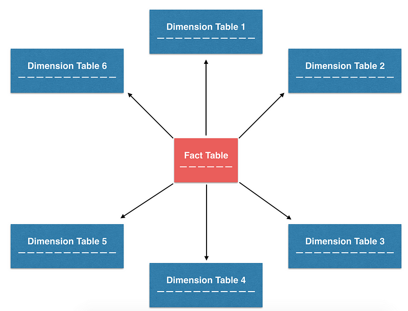
Among the many design patterns that try to balance this trade-off, one of the most commonly-used patterns, and the one we use at Airbnb, is called star schema. The name arose because tables organized in star schema can be visualized with a star-like pattern. This design focuses on building normalized tables, specifically fact and dimension tables. When needed, denormalized tables can be built from these smaller normalized tables. This design strives for a balance between ETL maintainability and ease of analytics.

Fact & Dimension Tables

To understand how to build denormalized tables from fact tables and dimension tables, we need to discuss their respective roles in more detail:

• Fact tables typically contain point-in-time transactional data. Each row in the table can be extremely simple and is often represented as a unit of transaction. Because of their simplicity, they are often the source of truth tables from which business metrics are derived. For example, at Airbnb, we have various fact tables that track transaction-like events such as bookings, reservations, alterations, cancellations, and more.
• Dimension tables typically contain slowly changing attributes of specific entities, and attributes sometimes can be organized in a hierarchical structure. These attributes are often called “dimensions”, and can be joined with the fact tables, as long as there is a foreign key available in the fact table. At Airbnb, we built various dimension tables such as users, listings, and markets that help us to slice and dice our data.

Below is a simple example of how fact tables and dimension tables (both are normalized tables) can be joined together to answer basic analytics question such as how many bookings occurred in the past week in each market. Shrewd users can also imagine that if additional metrics m_a, m_b, m_c and dimensions dim_x, dim_y, dim_z are projected in the final SELECT clause, a denormalized table can be easily built from these normalized tables.

Data Partitioning & Backfilling Historical Data

In an era where data storage cost is low and computation is cheap, companies now can afford to store all of their historical data in their warehouses rather than throwing it away. The advantage of such an approach is that companies can re-process historical data in response to new changes as they see fit.

Data Partitioning by Datestamp

With so much data readily available, running queries and performing analytics can become inefficient over time. In addition to following SQL best practices such as “filter early and often”, “project only the fields that are needed”, one of the most effective techniques to improve query performance is to partition data.

The basic idea behind data partitioning is rather simple — instead of storing all the data in one chunk, we break it up into independent, self-contained chunks. Data from the same chunk will be assigned with the same partition key, which means that any subset of the data can be looked up extremely quickly. This technique can greatly improve query performance.

In particular, one common partition key to use is datestamp (ds for short), and for good reason. First, in data storage system like S3, raw data is often organized by datestamp and stored in time-labeled directories. Furthermore, the unit of work for a batch ETL job is typically one day, which means new date partitions are created for each daily run. Finally, many analytical questions involve counting events that occurred in a specified time range, so querying by datestamp is a very common pattern. It is no wonder that datestamp is a popular choice for data partitioning!

Backfilling Historical Data

Another important advantage of using datestamp as the partition key is the ease of data backfilling. When a ETL pipeline is built, it computes metrics and dimensions forward, not backward. Often, we might desire to revisit the historical trends and movements. In such cases, we would need to compute metric and dimensions in the past — We called this process data backfilling.

Backfilling is so common that Hive built in the functionality of dynamic partitions, a construct that perform the same SQL operations over many partitions and perform multiple insertions at once. To illustrate how useful dynamic partitions can be, consider a task where we need to backfill the number of bookings in each market for a dashboard, starting from earliest_ds to latest_ds . We might do something like this:

The operation above is rather tedious, since we are running the same query many times but on different partitions. If the time range is large, this work can become quickly repetitive. When dynamic partitions are used, however, we can greatly simplify this work into just one query:

Notice the extra ds in the SELECT and GROUP BY clause, the expanded range in the WHERE clause, and how we changed the syntax from PARTITION (ds= '{{ds}}') to PARTITION (ds) . The beauty of dynamic partitions is that we wrap all the same work that is needed with a GROUP BY ds and insert the results into the relevant ds partitions all at once. This query pattern is very powerful and is used by many of Airbnb’s data pipelines. In a later section, I will demonstrate how one can write an Airflow job that incorporates backfilling logic using Jinja control flow.

The Anatomy of an Airflow Pipeline

Now that we have learned about the concept of fact tables, dimension tables, date partitions, and what it means to do data backfilling, let’s crystalize these concepts and put them in an actual Airflow ETL job.

Defining the Directed Acyclic Graph (DAG)

As we mentioned in the earlier post, any ETL job, at its core, is built on top of three building blocks: Extract, Transform, and Load. As simple as it might sound conceptually, ETL jobs in real life are often complex, consisting of many combinations of E, T, and L tasks. As a result, it is often useful to visualize complex data flows using a graph. Visually, a node in a graph represents a task, and an arrow represents the dependency of one task on another. Given that data only needs to be computed once on a given task and the computation then carries forward, the graph is directed and acyclic. This is why Airflow jobs are commonly referred to as “DAGs” (Directed Acyclic Graphs).

One of the clever designs about Airflow UI is that it allows any users to visualize the DAG in a graph view, using code as configuration. The author of a data pipeline must define the structure of dependencies among tasks in order to visualize them. This specification is often written in a file called the DAG definition file, which lays out the anatomy of an Airflow job.

Operators: Sensors, Operators, and Transfers

While DAGs describe how to run a data pipeline, operators describe what to do in a data pipeline. Typically, there are three broad categories of operators:

• Sensors: waits for a certain time, external file, or upstream data source
• Operators: triggers a certain action (e.g. run a bash command, execute a python function, or execute a Hive query, etc)
• Transfers: moves data from one location to another

Shrewd readers can probably see how each of these operators correspond to the Extract, Transform, and Load steps that we discussed earlier. Sensors unblock the data flow after a certain time has passed or when data from an upstream data source becomes available. At Airbnb, given that most of our ETL jobs involve Hive queries, we often used NamedHivePartitionSensors to check whether the most recent partition of a Hive table is available for downstream processing.

Operators trigger data transformations, which corresponds to the Transform step. Because Airflow is open-source, contributors can extend BaseOperator class to create custom operators as they see fit. At Airbnb, the most common operator we used is HiveOperator (to execute hive queries), but we also use PythonOperator (e.g. to run a Python script) and BashOperator (e.g. to run a bash script, or even a fancy Spark job) fairly often. The possibilities are endless here!

Finally, we also have special operators that Transfers data from one place to another, which often maps to the Load step in ETL. At Airbnb, we use MySqlToHiveTransfer or S3ToHiveTransfer pretty often, but this largely depends on one’s data infrastructure and where the data warehouse lives.

A Simple Example

Below is a simple example that demonstrate how to define a DAG definition file, instantiate a Airflow DAG, and define the corresponding DAG structure using the various operators we described above.

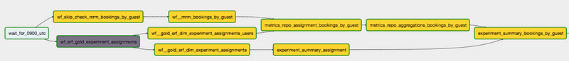
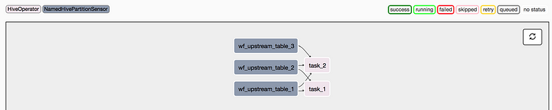
When the DAG is rendered, we see the following graph view:

ETL Best Practices To Follow

Like any craft, writing Airflow jobs that are succinct, readable, and scalable requires practice. On my first job, ETL to me was just a series of mundane mechanical tasks that I had to get done. I did not see it as a craft nor did I know the best practices. At Airbnb, I learned a lot about best practices and I started to appreciate good ETLs and how beautiful they can be. Below, I list out a non-exhaustive list of principles that good ETL pipelines should follow:

• Partition Data Tables: As we mentioned earlier, data partitioning can be especially useful when dealing with large-size tables with a long history. When data is partitioned using datestamps, we can leverage dynamic partitions to parallelize backfilling.

• Load Data Incrementally: This principle makes your ETL more modular and manageable, especially when building dimension tables from the fact tables. In each run, we only need to append the new transactions to the dimension table from previous date partition instead of scanning the entire fact history.

• Enforce Idempotency: Many data scientists rely on point-in-time snapshots to perform historical analysis. This means the underlying source table should not be mutable as time progresses, otherwise we would get a different answer. Pipeline should be built so that the same query, when run against the same business logic and time range, returns the same result. This property has a fancy name called Idempotency.
• Parameterize Workflow: Just like how templates greatly simplified the organization of HTML pages, Jinja can be used in conjunction with SQL. As we mentioned earlier, one common usage of Jinja template is to incorporate the backfilling logic into a typical Hive query. Stitch Fix has a very nice post that summarized how they use this technique for their ETL.

• Add Data Checks Early and Often: When processing data, it is useful to write data into a staging table, check the data quality, and only then exchange the staging table with the final production table. At Airbnb, we call this the stage-check-exchange paradigm. Checks in this 3-step paradigm are important defensive mechanisms — they can be simple checks such as counting if the total number of records is greater than 0 or something as complex as an anomaly detection system that checks for unseen categories or outliers.

• Build Useful Alerts & Monitoring System: Since ETL jobs can often take a long time to run, it’s useful to add alerts and monitoring to them so we do not have to keep an eye on the progress of the DAG constantly. Different companies monitor DAGs in many creative ways — at Airbnb, we regularly use EmailOperators to send alert emails for jobs missing SLAs. Other teams have used alerts to flag experiment imbalances. Yet another interesting example is from Zymergen where they report model performance metrics such as R-squared with a SlackOperator.

Many of these principles are inspired by a combination of conversations with seasoned data engineers, my own experience building Airflow DAGs, and readings from Gerard Toonstra’s ETL Best Practices with Airflow. For the curious readers, I highly recommend this following talk from Maxime:

Recap of Part II

In the second post of this series, we discussed star schema and data modeling in much more details. We learned the distinction between fact and dimension tables, and saw the advantages of using datestamps as partition keys, especially for backfilling. Furthermore, we dissected the anatomy of an Airflow job, and crystallized the different operators available in Airflow. We also highlighted best practices for building ETL, and showed how flexible Airflow jobs can be when used in conjunction with Jinja and SlackOperators. The possibilities are endless!

In the last post of the series, I will discuss a few advanced data engineering patterns — specifically, how to go from building pipelines to building frameworks. I will again use a few example frameworks that we used at Airbnb as motivating examples.

If you found this post useful, please visit Part I and stay tuned for Part III.

I want to appreciate Jason Goodman and Michael Musson for providing invaluable feedback to me

Slope Over Intercept

Exploring the intersections of data, engineering, and product management

Slope Over InterceptRobert Chang